Developing a Heat Vulnerability Index (HVI) is a multistep process drawing on multiple data inputs. Using composites of social, economic, and health related demographics along with temperature and vegetation variability, influenced by several studies, I created a Heat Vulnerability Index (HVI) to locate populations that are at an increased risk of heat stroke or other heat-related illnesses. The HVI was used in my main piece about Urban Heat Islands in the District.
Deriving the HVI begins with calculating average temperatures and NDVI for each census tract with in DC. Using NASA’s Landsat 8 data, it is possible to derive temperature from remotely senses satellite images. Landsat 8 collects data at various electromagnetic wavelengths. Temperature related data is collected as raster products under bands 10 and 11 (Thermal Infrared) at 100 meter resolutions. Raw reflectance, which is how the data is recorded, is not immediately useful. Reflectance must first be converted to radiance for each band, followed by a conversions to temperature, and finally averaging the values of each together. Below is the script used to derive temperature using the arcpy module within ArcMap.
Setting up variables
# Import arcpy module
import arcpy

# Band related local variables:
Band_10 = "LC08_L1TP_015033_20150817_20170226_01_T1_B10.TIF"
Band_11 = "LC08_L1TP_015033_20150817_20170226_01_T1_B11.TIF"
B10_Rad = "G:\\DC Policy Center\\Urban Heat Island\\Data\\Spatial Data\\Heat_Island.gdb\\B10_Rad.tif"
B10_Temp = "G:\\DC Policy Center\\Urban Heat Island\\Data\\Spatial Data\\Heat_Island.gdb\\B10_Temp.tif"
B11_Rad = "G:\\DC Policy Center\\Urban Heat Island\\Data\\Spatial Data\\Heat_Island.gdb\\B11_Rad.tif"
B11_Temp = "G:\\DC Policy Center\\Urban Heat Island\\Data\\Spatial Data\\Heat_Island.gdb\\B11_Temp.tif"
Final_Temperature = "G:\\DC Policy Center\\Urban Heat Island\\Data\\Spatial Data\\Heat_Island.gdb\\Temp_08_17_2015"

# Census related local variables:
final_temp_clip = "G:\\DC Policy Center\\Urban Heat
Island\\Data\\Spatial Data\\Heat_Island.gdb\\DC_Temp_08_17_15"
Census_Tract = "Census_Tract"
Temp_Vector = "G:\\DC Policy Center\\Urban Heat Island\\Data\\Spatial Data\\Heat_Island.gdb\\Temp_Points"
Neighborhood_Clusters = "Neighborhood_Clusters"
Temp_Vector_clip = "G:\\DC Policy Center\\Urban Heat Island\\Data\\Spatial Data\\Heat_Island.gdb\\Temp_Point_Extract"
Tract_Temp_Avg = "G:\\DC Policy Center\\Urban Heat Island\\Data\\Spatial Data\\Heat_Island.gdb\\CT_Temp_AVG"
Band conversions
# Band 10 to Radiance
arcpy.gp.RasterCalculator_sa("0.0003342 * " B10 " + 0.1", B10_Rad)
# Band 11 to Radiance
arcpy.gp.RasterCalculator_sa("0.0003342 * " B11 " + 0.1", B11_Rad)

# Band 10 Radiance to Temperature
arcpy.gp.RasterCalculator_sa("1321.08 / ln(774.89 / " B10_Rad " + 1) - 272.15", B10_Temp)
# Band 11 Radiance to Temperature
arcpy.gp.RasterCalculator_sa("1201.14 / ln(480.89 / " B11_Rad " + 1) - 272.15", B11_Temp)

# Average of Band 10 and 11 Temperatures
arcpy.gp.CellStatistics_sa("b11_temp;b10_temp", Final_Temperature, "MEAN", "DATA")
To gain the ability to compare the data with census demographics, this temperature data was converted to vector points. With vector points, values can be averaged through a spatial join with census tracts.
Variable conversions for analysis
# Clip Raster to DC Borders
arcpy.Clip_management(Temp_08_17_2015, "315900.112287067 4295387.04892389 334646.204049099 4318452.90089353", final_temp_clip, Census_Tract, "", "NONE", "NO_MAINTAIN_EXTENT")

# Convert Raster to Point Data
arcpy.RasterToPoint_conversion(final_temp_clip, Temp_Vector, "Value")

# Clip point data to exclude water features
arcpy.Clip_analysis(Temp_Vector, Neighborhood_Clusters, Temp_Vector_clip, "")

# Aggregate and Average temperatures by Census Tract
arcpy.SpatialJoin_analysis(Census_Tract, Temp_Vector_clip, Tract_Temp_Avg, "JOIN_ONE_TO_ONE", "KEEP_ALL", "GEOID \"GEOID\" true true false 11 Text 0 0 ,First,#,Census_Tract,GEOID,-1,-1;NAMELSAD \"NAMELSAD\" true true false 20 Text 0 0 ,First,#,Census_Tract,NAMELSAD,-1,-1;ALAND \"ALAND\" true true false 8 Double 0 0 ,First,#,Census_Tract,ALAND,-1,-1;AWATER \"AWATER\" true true false 8 Double 0 0 ,First,#,Census_Tract,AWATER,-1,-1;INTPTLAT \"INTPTLAT\" true true false 11 Text 0 0 ,First,#,Census_Tract,INTPTLAT,-1,-1;INTPTLON \"INTPTLON\" true true false 12 Text 0 0 ,First,#,Census_Tract,INTPTLON,-1,-1;N_Cluster \"N_Cluster\" true true false 50 Text 0 0 ,First,#,Census_Tract,N_Cluster,-1,-1;N_Name \"N_Name\" true true false 50 Text 0 0 ,First,#,Census_Tract,N_Name,-1,-1;Temp \"Temprature\" true true false 50 Double 0 0 ,Mean,#", "INTERSECT", "", "")
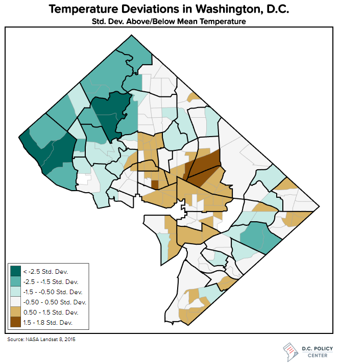
Temperature was converted to standard deviation of the mean, to indicate the range of variability throughout the city. In the map below, temperature deviations among census tracts is visualized. The hottest (0 to 1.8 Std. Dev neighborhoods include Trinidad, Ivy City, Eckington, and the southern extents of Logan Circle. On the cooler end of the spectrum (< -2.5 to 0 Std. Dev ), almost the entirety of the City west of Rock Creek Park was below the mean temperature. To put this into real temperature terms , if the average temperature of the city was 90˚F, the coolest areas of the city could be almost 10-12˚F cooler. This occurs regularly in neighbors such as Palisades, Foxhall Crescent and Forrest Hills. These neighborhoods are all located in N.W. D.C. and are characterized by their proximity to large forested stretches such as Rock Creek Park or Battery Kemble Park.
Normalized Difference Vegetation Index (NDVI), another key variable in the HVI, is also derived from Landsat 8 data. Instead of using bands 10 and 11, NDVI relies on bands 4 (Red) and 5(Near Infrared). NDVI is then calculated using the following formula. Similar to temperature, NDVI values were extracted from a raster formatted and averaged over census tracts. \[ NDVI = {NIR - Red \over NIR + Red} \] In addition to temperature and vegetation data, I extracted social and economic demographic data from the American Community Survey and Health data from the Center for Disease Control. Various factors were selected from both datasets and chosen due to previous studies having identified them as being particularly susceptible to heat related illnesses. Vulnerable populations include those who are:
- Below the poverty line,
- Don’t have a high school diploma,
- Without health insurance,
- Older than 65,
- Living alone,
- are not white,
- or experiencing persistently poor physical health.
From this data, I calculated the weighted influence of each demographic indicator along with temperature and NDVI to derive the HVI score for each census tract. Previous studies have weighted all factors equally. I did not follow this practice. The weights I applied to each input was subjective and based on my interpretation to which factors would lead to a greater vulnerability.
Applied weights
| Factor | Weight |
|---|---|
| Temperature deviation | 0.15 |
| % below poverty line | 0.15 |
| % experiencing persistently poor physical health | 0.15 |
| % over 65 and living alone | 0.15 |
| NDVI | 0.1 |
| % over 65 | 0.1 |
| % uninsured | 0.05 |
| % living alone | 0.05 |
| % not white | 0.03 |
| % no high school diploma | 0.02 |
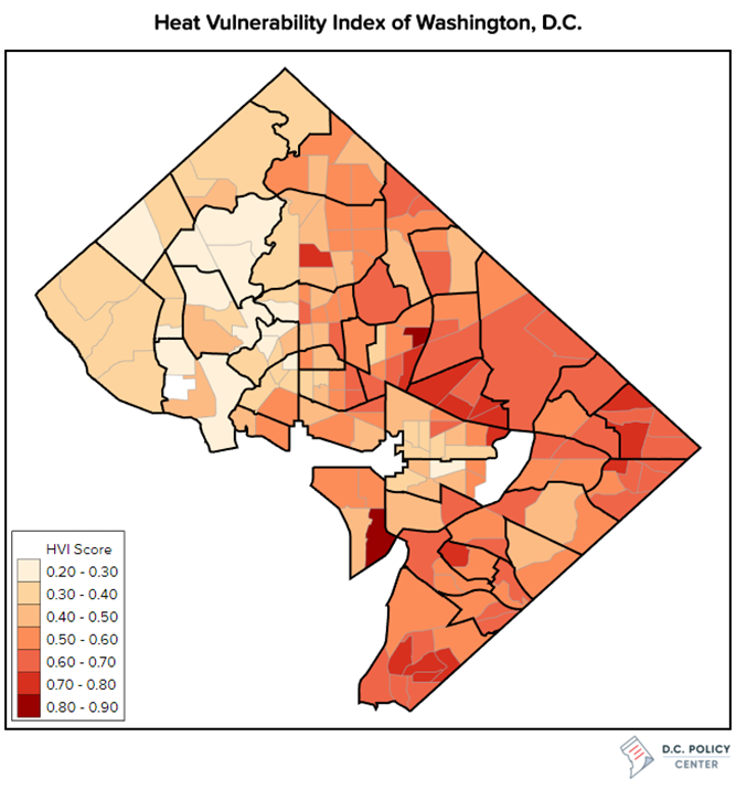
Mapping the final calculated HVI score, spatial patterns become apparent. The neighborhoods at highest risk of heat stroke or heat-related illnesses include those of Buzzard Point, Edgewood, and Washington Highlands. Those with the lowest risk are concentrated to the west of Rock Creek Park.
Final product
Combining the analysis into a final map produces a nice interactive carto.
About the data
Social and economic demographic data acquired from the U.S. Census Bureau’s American Community Survey, 2015. Health data acquired from the Center for Disease Control, 2014. Imagery used to derive temperature and NDVI values acquired from NASA’s Landsat 8 satellite and downloaded from the USGS’s Earth Explorer repository. You can find complete code for the analysis and visuals on my github page.